Reading and writing data

A short description of the post.

Load the R packages we will use

library(tidyverse)
library(here)
library(janitor)
library(skimr)

Download emissions per capita form Our World in Data into the directory for this post.
Assign the location of the file to file_csv. The data should be in the same directory as this file.

Read the data into R and assign it to emissions

file_csv <- here("_posts",
                 "2022-02-22-reading-and-writing-data",
                 "co-emissions-per-capita.csv")

emissions <- read_csv(file_csv)

Show the first 10 rows (observations of) emissions
```
emissions
```

# A tibble: 23,307 x 4
   Entity      Code   Year `Annual CO2 emissions (per capita)`
   <chr>       <chr> <dbl>                               <dbl>
 1 Afghanistan AFG    1949                              0.0019
 2 Afghanistan AFG    1950                              0.0109
 3 Afghanistan AFG    1951                              0.0117
 4 Afghanistan AFG    1952                              0.0115
 5 Afghanistan AFG    1953                              0.0132
 6 Afghanistan AFG    1954                              0.013 
 7 Afghanistan AFG    1955                              0.0186
 8 Afghanistan AFG    1956                              0.0218
 9 Afghanistan AFG    1957                              0.0343
10 Afghanistan AFG    1958                              0.038 
# ... with 23,297 more rows

Start with emiaaions data THEN

use clean_names from the janitor package to make the names easier to work with
assign the output to tidy_emissions
show the first 10 rows of tidy_emissions

tidy_emissions <- emissions %>% 
  clean_names()

tidy_emissions

# A tibble: 23,307 x 4
   entity      code   year annual_co2_emissions_per_capita
   <chr>       <chr> <dbl>                           <dbl>
 1 Afghanistan AFG    1949                          0.0019
 2 Afghanistan AFG    1950                          0.0109
 3 Afghanistan AFG    1951                          0.0117
 4 Afghanistan AFG    1952                          0.0115
 5 Afghanistan AFG    1953                          0.0132
 6 Afghanistan AFG    1954                          0.013 
 7 Afghanistan AFG    1955                          0.0186
 8 Afghanistan AFG    1956                          0.0218
 9 Afghanistan AFG    1957                          0.0343
10 Afghanistan AFG    1958                          0.038 
# ... with 23,297 more rows

Start with the tidy_emissions THEN

use filter to extract rows with year == 1988 THEN
use skim to calculate the descriptive statistics

tidy_emissions %>% 
  filter(year == 1988) %>% 
  skim()

Table 1: Data summary
Name	Piped data
Number of rows	217
Number of columns	4
_______________________
Column type frequency:
character	2
numeric	2
________________________
Group variables	None

Variable type: character

skim_variable	n_missing	complete_rate	min	max	empty	n_unique	whitespace
entity	0	1.00	4	32	0	217	0
code	12	0.94	3	8	0	205	0

Variable type: numeric

skim_variable	n_missing	complete_rate	mean	sd	p0	p25	p50	p75	p100	hist
year	0	1	1988.00	0.00	1988.00	1988.00	1988.00	1988.00	1988.00	▁▁▇▁▁
annual_co2_emissions_per_capita	0	1	5.06	5.87	0.01	0.56	2.76	8.11	29.56	▇▂▁▁▁

12 observations have a missing code. How are these observations diffrent?

start with tidy_emissions then extract rows with year == 1988 and are missing a code

tidy_emissions %>% 
  filter(year == 1988, is.na(code))

# A tibble: 12 x 4
   entity                     code   year annual_co2_emissions_per_ca~
   <chr>                      <chr> <dbl>                        <dbl>
 1 Africa                     <NA>   1988                         1.23
 2 Asia                       <NA>   1988                         2.00
 3 Asia (excl. China & India) <NA>   1988                         2.92
 4 EU-27                      <NA>   1988                         9.08
 5 EU-28                      <NA>   1988                         9.20
 6 Europe                     <NA>   1988                        11.0 
 7 Europe (excl. EU-27)       <NA>   1988                        13.5 
 8 Europe (excl. EU-28)       <NA>   1988                        14.3 
 9 North America              <NA>   1988                        14.3 
10 North America (excl. USA)  <NA>   1988                         5.17
11 Oceania                    <NA>   1988                        11.2 
12 South America              <NA>   1988                         2.04

Start with tidy_emissions THEN -use filter to extract rows with year == 1988 and Without missing codes THEN

use select to drop the `year`` variable THEN
Use rename to change the variable entity to country

assign the output to emissions_1988

emissions_1988 <- tidy_emissions %>% 
filter(year == 1988, !is.na(code)) %>% 
select(-year) %>% 
rename(country = entity)

Which 15 countries have the highest per_capita_co2_emissions?

-start with emissions_1988 THEN -use slice_max to extract the 15 rows with the per_capita_co2_emissions -assign the output to max_15_emitters

max_15_emitters <- emissions_1988 %>% 
  slice_max(annual_co2_emissions_per_capita, n = 15)

Which 15 countries have the lowest annual_co2_emissions_per_capita?

start with emissions_1988 then -use slice_min to extract the 15 rows with the lowest values assign the output to min_15_emitters

min_15_emitters <- emissions_1988 %>% 
  slice_min(annual_co2_emissions_per_capita, n = 15)

Use bind_rows to bind together the max_15_emitters and min_15_emitters assign the output to `max_min_15

max_min_15 <- bind_rows(max_15_emitters, min_15_emitters)

Export max_min_15 to 3 file formats

max_min_15 %>% write_csv("max_min_15.csv") # comma-separated values
max_min_15 %>% write_tsv("max_min_15.tsv") # tab separated
max_min_15 %>% write_delim("max_min_15.psv", delim = "|") #pipe-separated

Read the 3 file formats into R

max_min_15_csv <-  read_csv("max_min_15.csv") # comma-separated values
max_min_15_tsv <-  read_tsv("max_min_15.tsv") # tab separated
max_min_15_psv <-  read_delim("max_min_15.psv", delim = "|") #pipe-separated

Use setdiff to check for any differences among max_min_15_csv, max_min_15_tsv and max_min_15_psv

setdiff(max_min_15_psv, max_min_15_tsv)

# A tibble: 0 x 3
# ... with 3 variables: country <chr>, code <chr>,
#   annual_co2_emissions_per_capita <dbl>

Reorder country in max_min_15 for plotting and assign to max_min_15_plot_data -start with emissions_2019 THEN use mutate to reorder country according to annual_co2_emissions_per_capita

max_min_15_plot_data <- max_min_15 %>% 
  mutate(country = reorder(country, annual_co2_emissions_per_capita))

Plot ‘max_min_15_plot_data’

ggplot(data = max_min_15_plot_data,
   mapping = aes(x= annual_co2_emissions_per_capita, y = country))+
  geom_col()+
  labs(title = "The top 15 and bottom 15 per capita CO2 emissions",
   subtitle = "for 1988",
   x = NULL,
   y = NULL)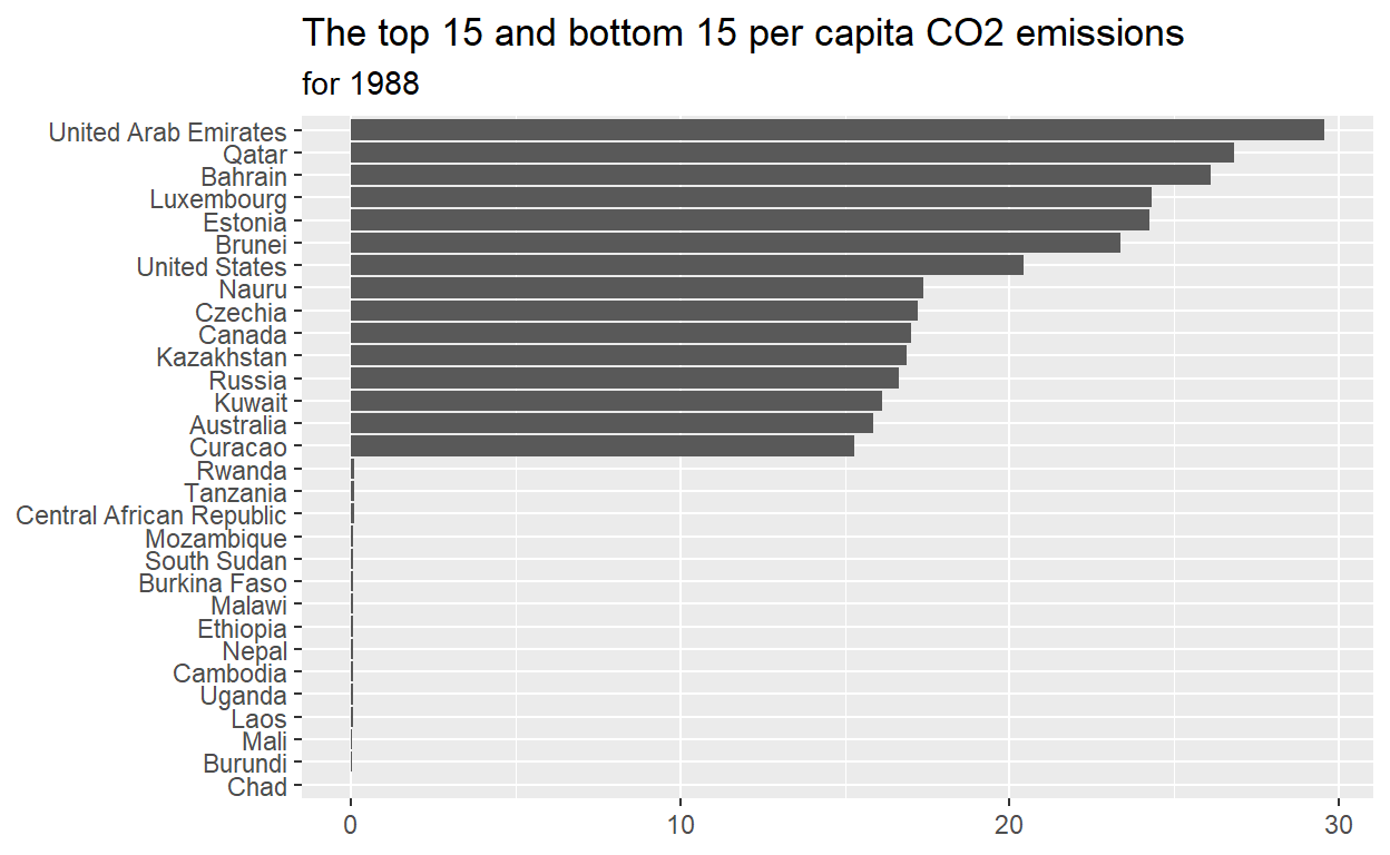

Save the plot dirextory with this post

ggsave(filename = "preview.png",
   path = here("_posts", "2022-02-22-reading-and-writing-data"))

18.Add preview.png to yaml chuck at the top of this file

preview: preview.png

Reading and writing data

Authors

Affiliations

Published

DOI

Footnotes