Steps 1-6

Load the R packages we will use.

library(tidyverse)
library(echarts4r) #install this package before using
library(hrbrthemes) #install this package before using

Read the data in the files, drug_cos.csv, health_cos.csv in the R and assign to the variables drug_cos and health_cos, respectively

drug_cos <- read.csv("https://estanny.com/static/week6/drug_cos.csv")
health_cos <- read_csv("https://estanny.com/static/week6/health_cos.csv")

Use glimpse to get a glimpse of the data

drug_cos %>% glimpse()

Rows: 104
Columns: 9
$ ticker       <chr> "ZTS", "ZTS", "ZTS", "ZTS", "ZTS", "ZTS", "ZTS"~
$ name         <chr> "Zoetis Inc", "Zoetis Inc", "Zoetis Inc", "Zoet~
$ location     <chr> "New Jersey; U.S.A", "New Jersey; U.S.A", "New ~
$ ebitdamargin <dbl> 0.149, 0.217, 0.222, 0.238, 0.182, 0.335, 0.366~
$ grossmargin  <dbl> 0.610, 0.640, 0.634, 0.641, 0.635, 0.659, 0.666~
$ netmargin    <dbl> 0.058, 0.101, 0.111, 0.122, 0.071, 0.168, 0.163~
$ ros          <dbl> 0.101, 0.171, 0.176, 0.195, 0.140, 0.286, 0.321~
$ roe          <dbl> 0.069, 0.113, 0.612, 0.465, 0.285, 0.587, 0.488~
$ year         <int> 2011, 2012, 2013, 2014, 2015, 2016, 2017, 2018,~

health_cos %>% glimpse()

Rows: 464
Columns: 11
$ ticker      <chr> "ZTS", "ZTS", "ZTS", "ZTS", "ZTS", "ZTS", "ZTS",~
$ name        <chr> "Zoetis Inc", "Zoetis Inc", "Zoetis Inc", "Zoeti~
$ revenue     <dbl> 4233000000, 4336000000, 4561000000, 4785000000, ~
$ gp          <dbl> 2581000000, 2773000000, 2892000000, 3068000000, ~
$ rnd         <dbl> 427000000, 409000000, 399000000, 396000000, 3640~
$ netincome   <dbl> 245000000, 436000000, 504000000, 583000000, 3390~
$ assets      <dbl> 5711000000, 6262000000, 6558000000, 6588000000, ~
$ liabilities <dbl> 1975000000, 2221000000, 5596000000, 5251000000, ~
$ marketcap   <dbl> NA, NA, 16345223371, 21572007994, 23860348635, 2~
$ year        <dbl> 2011, 2012, 2013, 2014, 2015, 2016, 2017, 2018, ~
$ industry    <chr> "Drug Manufacturers - Specialty & Generic", "Dru~

Which variables are the same in both data sets

names_drug <- drug_cos %>% names()
names_health <- health_cos %>% names()
intersect(names_drug, names_health)

[1] "ticker" "name"   "year"

Select subset of variables to work with

For drug_cos select (in this order): ticker, year, revenue, gp, industry
Extract observations for 2018
Assign output to drug_subset
For health_cos select (in this order): ticker, year, revenue, gp, industry
Extract observations for 2018
Assign output to health_subset

drug_subset <- drug_cos %>% 
  select(ticker, year, grossmargin) %>% 
  filter(year == 2018)
health_subset  <- health_cos  %>%
  select(ticker, year, revenue, gp, industry)  %>% 
  filter(year == 2018)

Keep all the rows and columns drug_subset join with columns in health_subset

drug_subset %>% left_join(health_subset)

   ticker year grossmargin     revenue          gp
1     ZTS 2018       0.672  5825000000  3914000000
2    PRGO 2018       0.387  4731700000  1831500000
3     PFE 2018       0.790 53647000000 42399000000
4     MYL 2018       0.350 11433900000  4001600000
5     MRK 2018       0.681 42294000000 28785000000
6     LLY 2018       0.738 24555700000 18125700000
7     JNJ 2018       0.668 81581000000 54490000000
8    GILD 2018       0.781 22127000000 17274000000
9     BMY 2018       0.710 22561000000 16014000000
10   BIIB 2018       0.865 13452900000 11636600000
11   AMGN 2018       0.827 23747000000 19646000000
12    AGN 2018       0.861 15787400000 13596000000
13   ABBV 2018       0.764 32753000000 25035000000
                                   industry
1  Drug Manufacturers - Specialty & Generic
2  Drug Manufacturers - Specialty & Generic
3              Drug Manufacturers - General
4  Drug Manufacturers - Specialty & Generic
5              Drug Manufacturers - General
6              Drug Manufacturers - General
7              Drug Manufacturers - General
8              Drug Manufacturers - General
9              Drug Manufacturers - General
10             Drug Manufacturers - General
11             Drug Manufacturers - General
12             Drug Manufacturers - General
13             Drug Manufacturers - General

Question: join_ticker

Start with drug_cos
Extract observations for the ticker BIIB from drug_cos
Assign output to the variable drug_cos_subset

drug_cos_subset <- drug_cos %>% 
  filter(ticker == "BIIB")

Display drug_cos_subset

drug_cos_subset

  ticker       name             location ebitdamargin grossmargin
1   BIIB Biogen Inc Massachusetts; U.S.A        0.404       0.908
2   BIIB Biogen Inc Massachusetts; U.S.A        0.402       0.901
3   BIIB Biogen Inc Massachusetts; U.S.A        0.432       0.876
4   BIIB Biogen Inc Massachusetts; U.S.A        0.475       0.879
5   BIIB Biogen Inc Massachusetts; U.S.A        0.493       0.885
6   BIIB Biogen Inc Massachusetts; U.S.A        0.491       0.871
7   BIIB Biogen Inc Massachusetts; U.S.A        0.495       0.867
8   BIIB Biogen Inc Massachusetts; U.S.A        0.511       0.865
  netmargin   ros   roe year
1     0.245 0.333 0.204 2011
2     0.250 0.335 0.211 2012
3     0.269 0.355 0.233 2013
4     0.302 0.404 0.294 2014
5     0.330 0.437 0.321 2015
6     0.323 0.431 0.322 2016
7     0.207 0.407 0.209 2017
8     0.329 0.435 0.334 2018

Use left_join to combine the rows and columns of drug_cos_subset with the columns of health_cos
Assign the output to combo_df

combo_df <- drug_cos_subset %>% 
  left_join(health_cos)

Display combo_df

combo_df

  ticker       name             location ebitdamargin grossmargin
1   BIIB Biogen Inc Massachusetts; U.S.A        0.404       0.908
2   BIIB Biogen Inc Massachusetts; U.S.A        0.402       0.901
3   BIIB Biogen Inc Massachusetts; U.S.A        0.432       0.876
4   BIIB Biogen Inc Massachusetts; U.S.A        0.475       0.879
5   BIIB Biogen Inc Massachusetts; U.S.A        0.493       0.885
6   BIIB Biogen Inc Massachusetts; U.S.A        0.491       0.871
7   BIIB Biogen Inc Massachusetts; U.S.A        0.495       0.867
8   BIIB Biogen Inc Massachusetts; U.S.A        0.511       0.865
  netmargin   ros   roe year     revenue          gp        rnd
1     0.245 0.333 0.204 2011  5048634000  4581854000 1219602000
2     0.250 0.335 0.211 2012  5516461000  4970967000 1334919000
3     0.269 0.355 0.233 2013  6932200000  6074500000 1444100000
4     0.302 0.404 0.294 2014  9703300000  8532300000 1893400000
5     0.330 0.437 0.321 2015 10763800000  9523400000 2012800000
6     0.323 0.431 0.322 2016 11448800000  9970100000 1973300000
7     0.207 0.407 0.209 2017 12273900000 10643900000 2253600000
8     0.329 0.435 0.334 2018 13452900000 11636600000 2597200000
   netincome      assets liabilities   marketcap
1 1234428000  9049604000  2622617000 26733054258
2 1380033000 10130118000  3166323000 34630691473
3 1862300000 11863335000  3242497000 66038521266
4 2934800000 14314700000  3500700000 80162952906
5 3547000000 19504800000 10129900000 68286367442
6 3702800000 22876800000 10748200000 61699770755
7 2539100000 23652600000 11054500000 67370207502
8 4430700000 25288900000 12257300000 60630142487
                      industry
1 Drug Manufacturers - General
2 Drug Manufacturers - General
3 Drug Manufacturers - General
4 Drug Manufacturers - General
5 Drug Manufacturers - General
6 Drug Manufacturers - General
7 Drug Manufacturers - General
8 Drug Manufacturers - General

Note: the variables ticker, name, location and industry are the same for all the observations

Assign the company name to co_name

co_name <- combo_df %>% 
  distinct(name) %>% 
  pull()

Assign the company location to co_location

co_location <- combo_df %>% 
  distinct(location) %>% 
  pull()

Assign the industry to co_industry group

co_industry <- combo_df %>% 
  distinct(industry) %>% 
  pull()

Put the r inline commands used in the blanks below. When you knit the document the results of the commands will be displayed in your text.

The company Biogen Inc is located in Massachusetts; U.S.A and is a member of the Drug Manufacturers - General industry group.

Start with combo_df
Select variables (in this order): year, grossmargin, netmargin,revenue, gp, netincome
Assign the output to combo_df_subset

combo_df_subset <- combo_df %>% 
  select(year, grossmargin, netmargin, 
  revenue, gp, netincome)

Display combo_df_subset

`combo_df_subset`

  year grossmargin netmargin     revenue          gp  netincome
1 2011       0.908     0.245  5048634000  4581854000 1234428000
2 2012       0.901     0.250  5516461000  4970967000 1380033000
3 2013       0.876     0.269  6932200000  6074500000 1862300000
4 2014       0.879     0.302  9703300000  8532300000 2934800000
5 2015       0.885     0.330 10763800000  9523400000 3547000000
6 2016       0.871     0.323 11448800000  9970100000 3702800000
7 2017       0.867     0.207 12273900000 10643900000 2539100000
8 2018       0.865     0.329 13452900000 11636600000 4430700000

Create the variable grossmargin_check to compare with the variable grossmargin. They should be equal. -grossmargin_check = gp / revenue
Create the variable close_enough to check that the absolute value of the difference between grossmargin_check and grossmargin is less than 0.001

combo_df_subset  %>% 
  mutate(grossmargin_check = gp / revenue,
  close_enough = abs(grossmargin_check - grossmargin) < 0.001)

  year grossmargin netmargin     revenue          gp  netincome
1 2011       0.908     0.245  5048634000  4581854000 1234428000
2 2012       0.901     0.250  5516461000  4970967000 1380033000
3 2013       0.876     0.269  6932200000  6074500000 1862300000
4 2014       0.879     0.302  9703300000  8532300000 2934800000
5 2015       0.885     0.330 10763800000  9523400000 3547000000
6 2016       0.871     0.323 11448800000  9970100000 3702800000
7 2017       0.867     0.207 12273900000 10643900000 2539100000
8 2018       0.865     0.329 13452900000 11636600000 4430700000
  grossmargin_check close_enough
1         0.9075433         TRUE
2         0.9011152         TRUE
3         0.8762730         TRUE
4         0.8793194         TRUE
5         0.8847619         TRUE
6         0.8708424         TRUE
7         0.8671979         TRUE
8         0.8649882         TRUE

Create the variable netmargin_check to compare with the variable netmargin. They should be equal.
Create the variable close_enough to check that the absolute value of the difference between netmargin_check and netmargin is less than 0.001

combo_df_subset  %>% 
  mutate(netmargin_check = netincome / revenue,
  close_enough = abs(netmargin_check - netmargin) < 0.001)

  year grossmargin netmargin     revenue          gp  netincome
1 2011       0.908     0.245  5048634000  4581854000 1234428000
2 2012       0.901     0.250  5516461000  4970967000 1380033000
3 2013       0.876     0.269  6932200000  6074500000 1862300000
4 2014       0.879     0.302  9703300000  8532300000 2934800000
5 2015       0.885     0.330 10763800000  9523400000 3547000000
6 2016       0.871     0.323 11448800000  9970100000 3702800000
7 2017       0.867     0.207 12273900000 10643900000 2539100000
8 2018       0.865     0.329 13452900000 11636600000 4430700000
  netmargin_check close_enough
1       0.2445073         TRUE
2       0.2501664         TRUE
3       0.2686449         TRUE
4       0.3024538         TRUE
5       0.3295305         TRUE
6       0.3234225         TRUE
7       0.2068699         TRUE
8       0.3293491         TRUE

Question: summarize_industry
Fill in the blanks
Put the command you use in the Rchunks in the Rmd file for this quiz
Use the health_cos data
For each industry calculate
mean_netmargin_percent = mean(netincome / revenue) * 100
median_netmargin_percent = median(netincome / revenue) * 100
Min_netmargin_percent = min(netincome / revenue) * 100
max_netmargin_percent = max(netincome / revenue) * 100

health_cos  %>% 
  group_by(industry)  %>% 
  summarize(mean_netmargin_percent = mean(netincome / revenue) * 100,
            median_netmargin_percent = median(netincome / revenue) * 100,
            Min_netmargin_percent = min(netincome / revenue) * 100,
            max_netmargin_percent = max(netincome / revenue) * 100
  )

# A tibble: 9 x 5
  industry          mean_netmargin_~ median_netmargi~ Min_netmargin_p~
  <chr>                        <dbl>            <dbl>            <dbl>
1 Biotechnology                -4.66             7.62         -197.   
2 Diagnostics & Re~            13.1             12.3             0.399
3 Drug Manufacture~            19.4             19.5           -34.9  
4 Drug Manufacture~             5.88             9.01          -76.0  
5 Healthcare Plans              3.28             3.37           -0.305
6 Medical Care Fac~             6.10             6.46            1.40 
7 Medical Devices              12.4             14.3           -56.1  
8 Medical Distribu~             1.70             1.03           -0.102
9 Medical Instrume~            12.3             14.0           -47.1  
# ... with 1 more variable: max_netmargin_percent <dbl>

Mean_netmargin_percent for the industry Medical Care Facilities is 6.10%
Medican_net_margin_percent for the industry Medical Care Facilities is 6.46%
min_netmargin_percent for the industry Medical Care Facilities 1.40%
max_netmargin_percent for the industry Medical Care Facilities 8.30%

Question: inline_ticker

Fill in the blanks
Use the health_cos data
Extract observations for the ticker BMY from health_cos and assign to the variable health_cos_subset

health_cos_subset  <- health_cos  %>% 
  filter(ticker == "BMY")

Display health_cos_subset

health_cos_subset

# A tibble: 8 x 11
  ticker name     revenue      gp    rnd netincome  assets liabilities
  <chr>  <chr>      <dbl>   <dbl>  <dbl>     <dbl>   <dbl>       <dbl>
1 BMY    Bristol~ 2.12e10 1.56e10 3.84e9    3.71e9 3.30e10 17103000000
2 BMY    Bristol~ 1.76e10 1.30e10 3.90e9    1.96e9 3.59e10 22259000000
3 BMY    Bristol~ 1.64e10 1.18e10 3.73e9    2.56e9 3.86e10 23356000000
4 BMY    Bristol~ 1.59e10 1.19e10 4.53e9    2.00e9 3.37e10 18766000000
5 BMY    Bristol~ 1.66e10 1.27e10 5.92e9    1.56e9 3.17e10 17324000000
6 BMY    Bristol~ 1.94e10 1.45e10 5.01e9    4.46e9 3.37e10 17360000000
7 BMY    Bristol~ 2.08e10 1.47e10 6.48e9    1.01e9 3.36e10 21704000000
8 BMY    Bristol~ 2.26e10 1.60e10 6.34e9    4.92e9 3.50e10 20859000000
# ... with 3 more variables: marketcap <dbl>, year <dbl>,
#   industry <chr>

In the console, type ?distinct. Go to the help pane to see what distinct does
In the console, type ?pull. Go to the help pane to see what pull does

Run the code below

health_cos_subset  %>% 
  distinct(name) %>%  
  pull(name)

[1] "Bristol Myers Squibb Co"

Assign the output to co_name

co_name  <- health_cos_subset  %>% 
  distinct(name) %>% 
  pull(name)

You can take output from your code and include it in your text.

The name of the company with ticker BMY is Bristol Myers Squibb Co

In following chunk

Assign the company’s industry group to the variable co_industry

co_industry  <- health_cos_subset  %>% 
  distinct(industry) %>% 
  pull()

This is outside the R chunk. Put the r inline commands used in the blanks below. When you knit the document the results of the commands will be displayed in your text.

The company Bristol Myers Squibb Co is a member of the Drug Manufacturers - General group.

Steps 7-11

Prepare the data for the plots

-start with health_cos THEN -group_by industry THEN -calculate the median research and development expenditure as a percent of revenue by industry -assign the output to df

df <- health_cos  %>% 
  group_by(industry)  %>%
  summarize(med_rnd_rev = median(rnd/revenue))

Use glimpse to glimpse the data for the plots

df  %>% glimpse()

Rows: 9
Columns: 2
$ industry    <chr> "Biotechnology", "Diagnostics & Research", "Drug~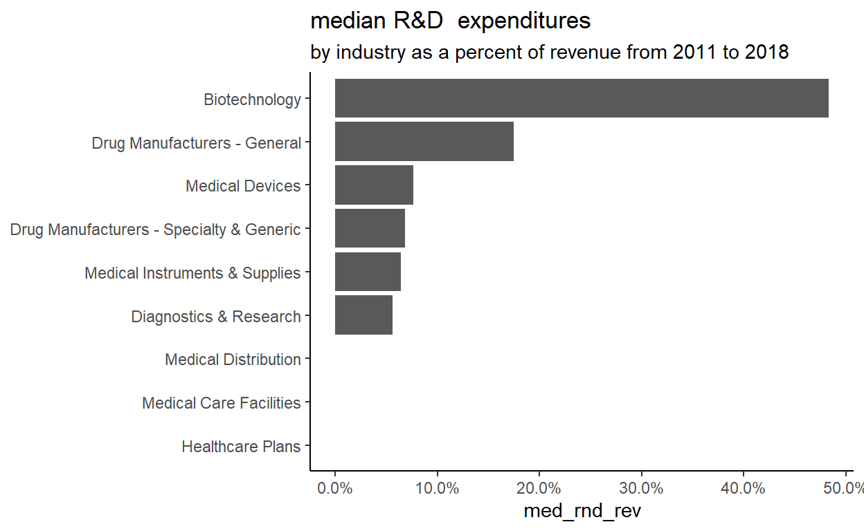
$ med_rnd_rev <dbl> 0.48317287, 0.05620271, 0.17451442, 0.06851879, ~

Create a static bar chart

use ggplot to initialize the chart
data is df
the variable industry is mapped to the x-axis
- reorder it based the value of med_rnd_rev
the variable med_rnd_rev is mapped to the y-axis
add a bar chart using geom_col
use scale_y_continuous to label the y-axis with percent
use coord_flip() to flip the coordinates
use labs to add title, subtitle and remove x and y-axes
use theme_ipsum() from the hrbrthemes package to improve the theme

ggplot(data = df,
       mapping = aes(
       x = reorder(industry, med_rnd_rev ),
       y = med_rnd_rev
       )) +
  geom_col() +
  scale_y_continuous(labels = scales::percent) +
  coord_flip() +
  labs(
    title = "median R&D  expenditures",
    subtitle = "by industry as a percent of revenue from 2011 to 2018",
    x = NULL, Y = NULL) +
  theme_classic()

Save the previous plot to preview.png and add to the yaml chunk at the top

ggsave(filename = "preview.png", 
       path = here::here("_posts", "2022-03-08-joining-data"))

Create an interactive bar chart using the package [echarts4r]

start with the data df
use arrange to reorder med_rnd_rev
use e_charts to initialize a chart - the variable industry is mapped to the x-axis
add a bar chart using e_bar with the values of med_rnd_rev
use e_flip_coords() to flip the coordinates
use e_title to add the title and the subtitle
use e_legend to remove the legends
use e_x_axis to change format of labels on x-axis to percent
use e_y_axis to remove labels on y-axis-
use e_theme to change the theme. Find more themes here

df  %>% 
  arrange(med_rnd_rev)  %>%
  e_charts(
    x = industry
    )  %>% 
  e_bar(
    serie = med_rnd_rev, 
    name = "median"
    )  %>%
  e_flip_coords()  %>% 
  e_tooltip()  %>% 
  e_title(
    text = "Median industry R&D expenditures", 
    subtext = "by industry as a percent of revenue from 2011 to 2018",
    left = "center") %>% 
  e_legend(FALSE) %>% 
  e_x_axis(
    formatter = e_axis_formatter("percent", digits = 0)
    )  %>%
  e_y_axis(
    show = FALSE
  )  %>% 
  e_theme("infographic")

Joining data

Steps 1-6

Question: join_ticker

Question: inline_ticker

Steps 7-11